`
Yuma-2 Seismometer
Yuma-2 Force Balance Vertical (FBV)
Seismometer Project
This page documents my experience building and operating a very
sensitive amateur seismometer, called Yuma-2. This instrument was
designed by Dave Nelson and Brett Nordgren, and is the second in a
series of three designs. First came Inyo, then Yuma, and most recently
Napa. At the time I started building, Napa was still experimental, and
Yuma was recommended as the most mature design, and the best one to
begin with. These are extraordinary instruments, for their
capabilities and their well thought out
mechanical and electrical design. I did not know much about
seismometers or seismology when I began this journey, and I've been
throughly impressed with the work and results that this small community
of developers has achieved.
I wanted a project that was substantial, challenging, required high
precision, and would allow me to learn some machining skills. I wanted
to build something that measures some aspect of the world around us,
sensing things that go unnoticed by most people. The Yuma turned out to
be a perfect choice.
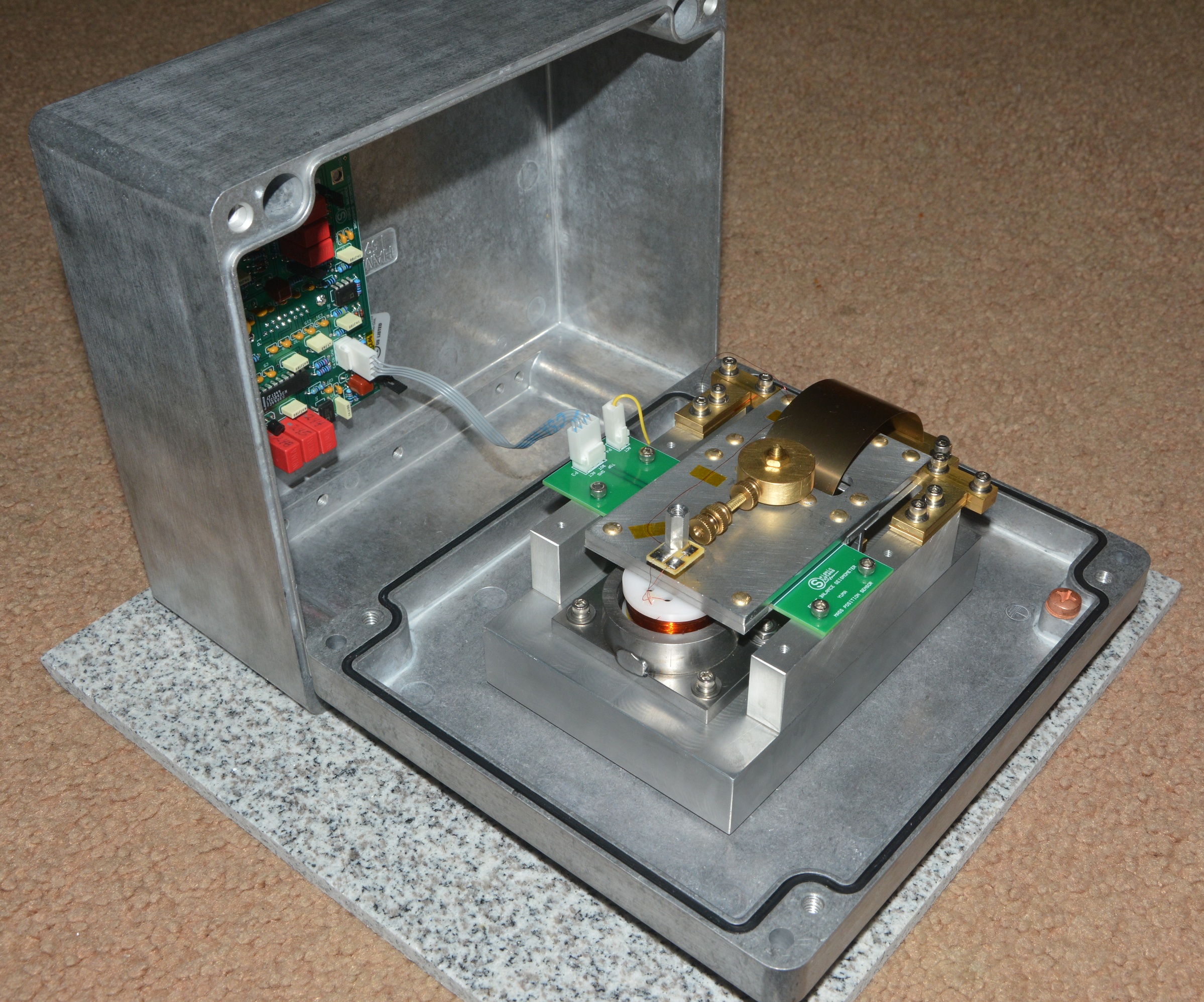
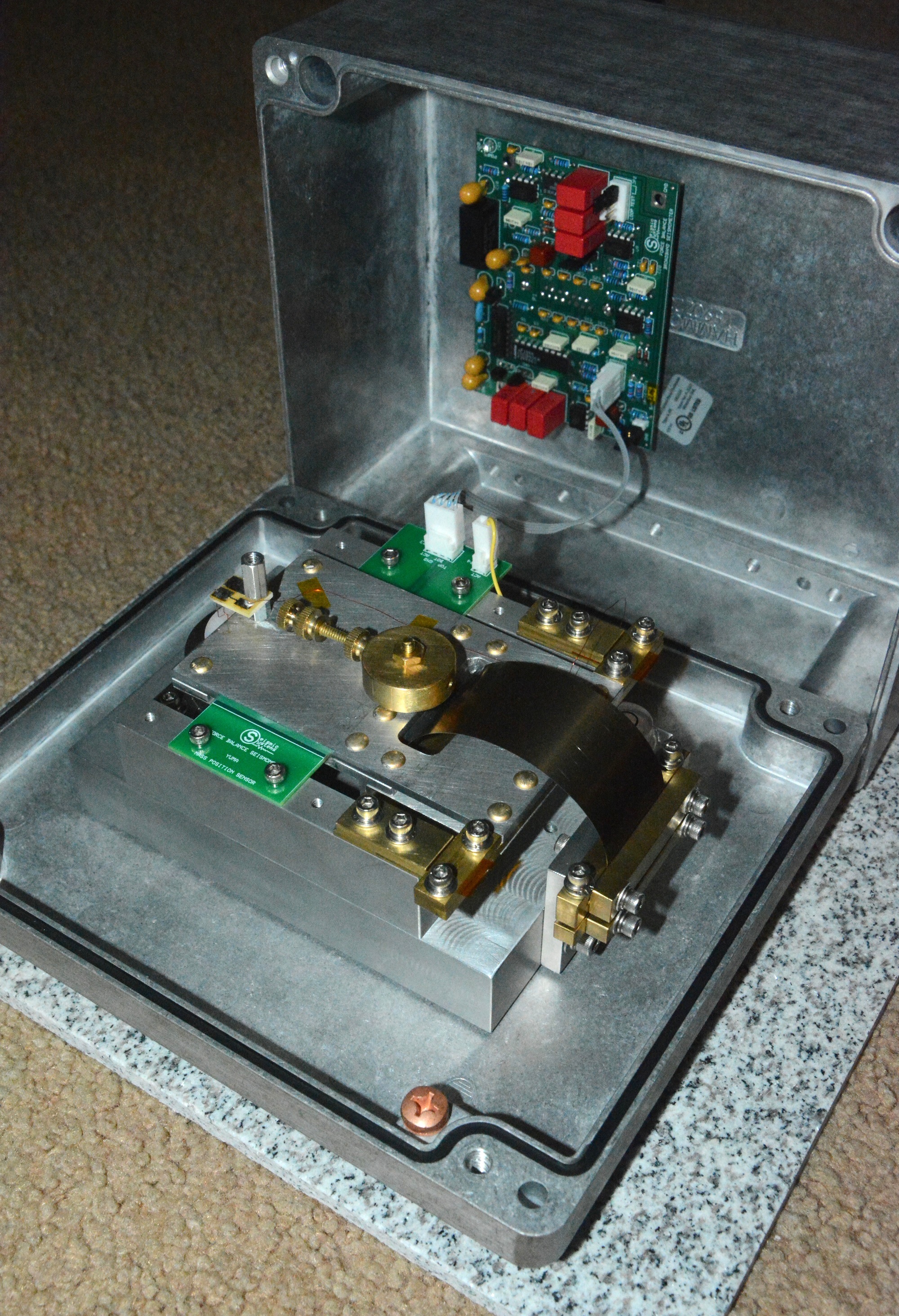
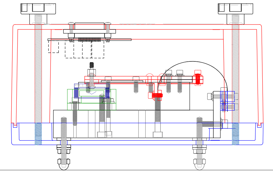
Seismometer
The instrument itself is relatively small, fitting in a case that is about 23
x 20 x 14 cm. It comprises a horizontal boom suspended by a leaf spring,
with a differential-capacitive position sensor and voice-coil actuator.
Trim weights are adjusted to set the rest position of the boom assembly
at the midpoint of travel, and to align the sensitive axis with the
vertical. Any disturbance in the boom position is sensed and amplified.
This signal is fed into an analog PID
(proportional-integral-differential) control circuit where it generates
a control signal to drive the voice coil actuator to oppose the
disturbance. This feedback loop keeps the boom nearly perfectly centered at
all times. Careful filtering is done to tailor the frequency response
of the system. The high gain of the feedback loop compensates for the
natural limitations of the mechanical system. The result is an
instrument that can detect ground velocity with low noise over a
wide range of frequencies, from a few milliHertz to over 30 Hz.
Sensitivity is impressive. Not having had much exposure to seismology
or the instruments that professionals use, I couldn't believe the
numbers when I first heard them. Properly installed at a good site,
this instrument can detection motions
of a few tens of nanometers/sec. Coming from the world of electronics where
cutting-edge integrated circuits are fabricated at similar nanometer
scales, and considering the cost and complexity of the instruments that
operate at these scales, I was amazed that an amatuer could build
an instrument with such sensitivity.
This level of sensitivity demands attention to detail. All
manner of secondary effects come into play as sources of noise which
obscure these slight movements. With the seismometer out in the
open, even in a quiet room with still air, imperceptable air currents
buffet the boom causing it to move up and down at a microscopic scale.
As we know, the atmospheric pressure around us changes slightly.
Pressure and temperature changes cause air density to change. The
aluminum and brass that comprise the boom have some amount of boyuancy
in air. Of course, its not enough for them to float off the table,
but it is enough for them to weigh slightly less in dense
air than they do in thin air. This difference is detectable by the
instrument. So air pressure and humidity must be stabilized. The
seismometer is mounted inside of an airtight case. But, the changing
atmospheric pressure causes the walls of the case to warp ever so
slightly. If care is not taken, some of this force would be transferred
to the base plate of the instrument, causing it to warp ever so
slightly. With the sensitivity of this instrument, such minor
deviations would show up in the data. So Dave and Brett designed an
ingeneous and effective implementation of a 'warpless' base to avoid
this problem.
The leaf spring, made of 17-7 stainless alloy, was specially heat
treated (precipitation hardended) to stabilize it over the long term.
Without that step, small pops could show up in the data, as various
metallic domains in the spring relaxed under the tension.
Air itself is a viscous fluid, and it will oppose the motion of a
plate, like that of the boom against the capacitive position sensor. So
a network of holes were designed into the PCB to allow that air an
escape route when the boom moves up and down a few microns.
The electronics are designed to be very low-noise. Chosing the best
components for these designs was not a simple matter of looking at
datasheet specs. The designers simulated, tested, and characterized these circuits for
the specific regime where they would be operating, to find those
op-amps, capacitors, and other components that were best suited for the
task at hand. Flicker-noise is a common problem in low-frequency
circuits, and the chosen amplifiers have very low 1/f noise
at the frequencies of interest, without having significant temperature effects,
or input bias currents, or offset drift. Film capacitors were chosen in
the signal processing chain for high linearity, absence of
piezoelectric effects, and minimal capcitance change with applied bias.
After PCB assembly, thorough cleaning of flux residue ensures no
leakage currents that might increase over time and degrade the
performance of high-impedance circuits.
There are literally dozens of small effects that must be understood by
the designers and carefully addressed in the design. It's clear that
these guys have an amazing amount of practical hands on experience and
knowledge in this area. And they've been a pleasure to work with.
I built Yuma-2 mechanical revision 4.3, electrical revision 4.0. Click here for:
Many of the documents and information on this site were taken from Brett's website, and others.
Here's how the Yuma compares to several professional instruments:
|
Yuma2
|
Trillium | STS-1
|
STS-2
|
Guralp CMG3
|
Category
|
Velocity broadband
|
Velocity broadband | Velocity very broadband
|
Velocity very broadband |
Velocity very broadband |
Flat response
|
20 mHz - 30 Hz
|
33 mHz - 50 Hz | 2.7 mHz - 10 Hz
|
8.3 mHz - 50 Hz
|
10 mHz - 50 Hz
|
Axes
|
1
|
3 | 1
|
3
|
3
|
Generator constant
|
1344 Vs/m
|
1500 Vs/m | 2 x 1200 Vs/m
|
2 x 750 Vs/m
|
2 x 750 Vs/m
|
Operational range
|
+/- 15 mm/s
|
+/- 5 mm/s | +/- 8 mm/s
|
+/- 13 mm/s
|
+/- 13 mm/s
|
Size
|
23 x 20 x 14 cm
|
22 x 18 cm | 12 x 17 x 18 cm
|
23 x 26 cm
|
17 x 37 cm
|
Weight
|
4.8 kg
|
11 kg | 4 kg |
13 kg
|
14 kg
|
Power
|
1.1 W
|
0.4 W | 3.5 W
|
0.8 W
|
0.75 W
|
Refer to some of Brett's documents for details on the theory of operation:
An excellent free text on seismology is the New Manual of Seismological Observatory Practice, consisting of chapters, datasheets, downloadable programs, and more.
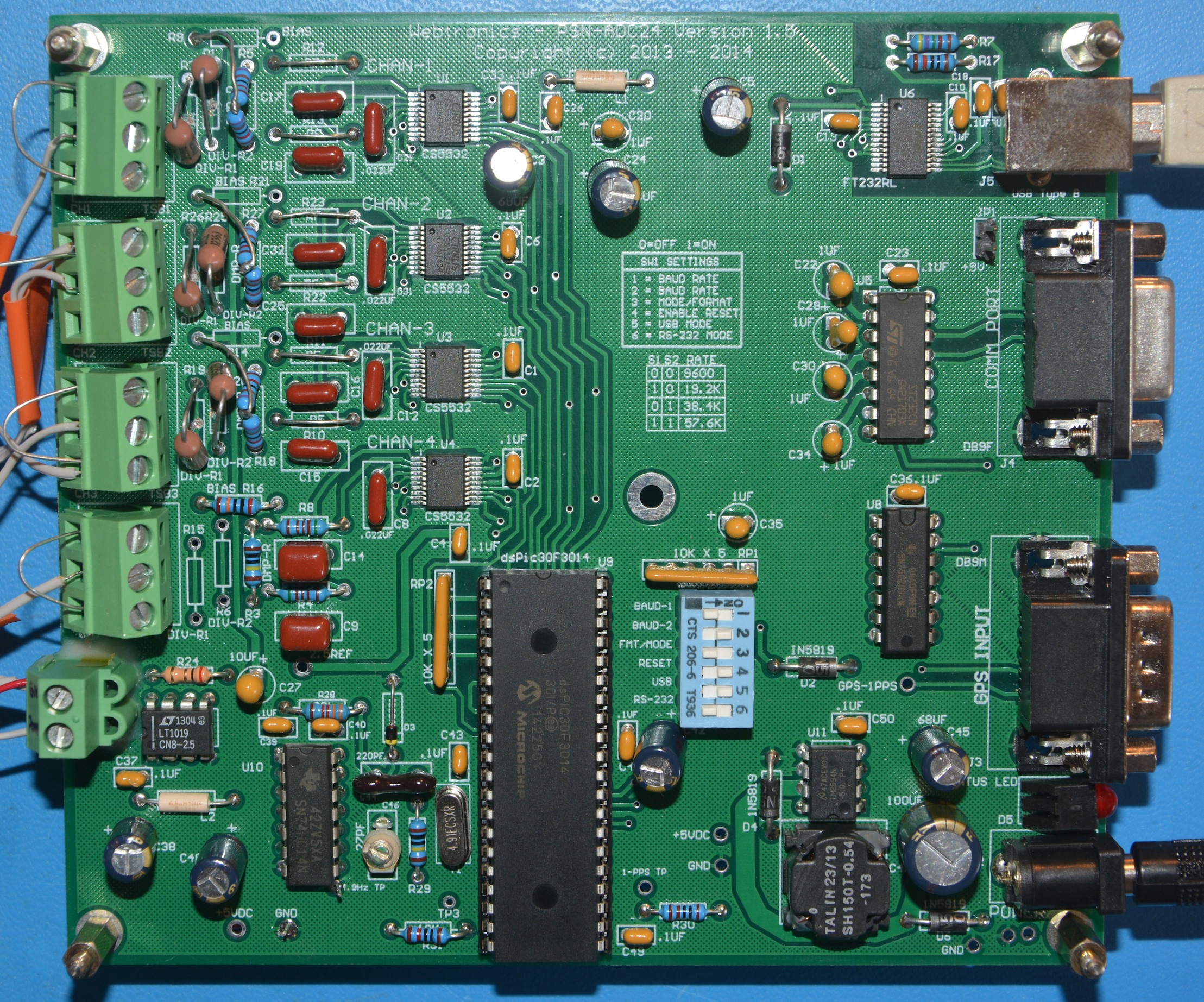
ADC
I purchased from Webtronics, Larry Cochrane's PSN-ADC24,
a four channel 24-bit low noise ADC board with USB/Serial interface.
This is a good board at a reasonable price, and it's
specifically designed for seismology applications. It integrates easily
with two pieces of seismology software, widely used by the community,
WinSDR and WinQuake.
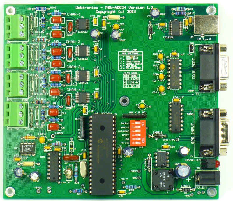
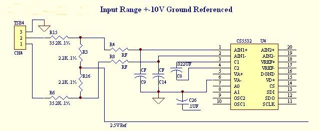
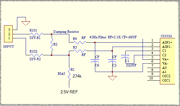
I'm using board version 1.5. Larry kindly configured the channels with different voltage dividers that I requested:
- CH1, 2, 3: +/-10V range - used to measure High and Low gain channels and Centering Force
- Divider ratio = 17.0
- R1, R2, R25, R26, R19 = 35.2 K
- R5, R18, R27 = 2.20K + 2.20K
- Rf = 5.1K, Cf = 0.1 uF
- R12, R13, R22, R23, R10, R11 = 0
- photos here and here
- CH4: +/- 2.5V range (biased at 2.5V midpoint, really 0 to 5V input) - used to measure temperature.
- Divider ratio = 1.0
- Rf = 5.1K, Cf = 0.68 uF, DIV-R1 = DIV-R2 = 0, R2 = open
- R15, R6 = open
- R3 = 1M
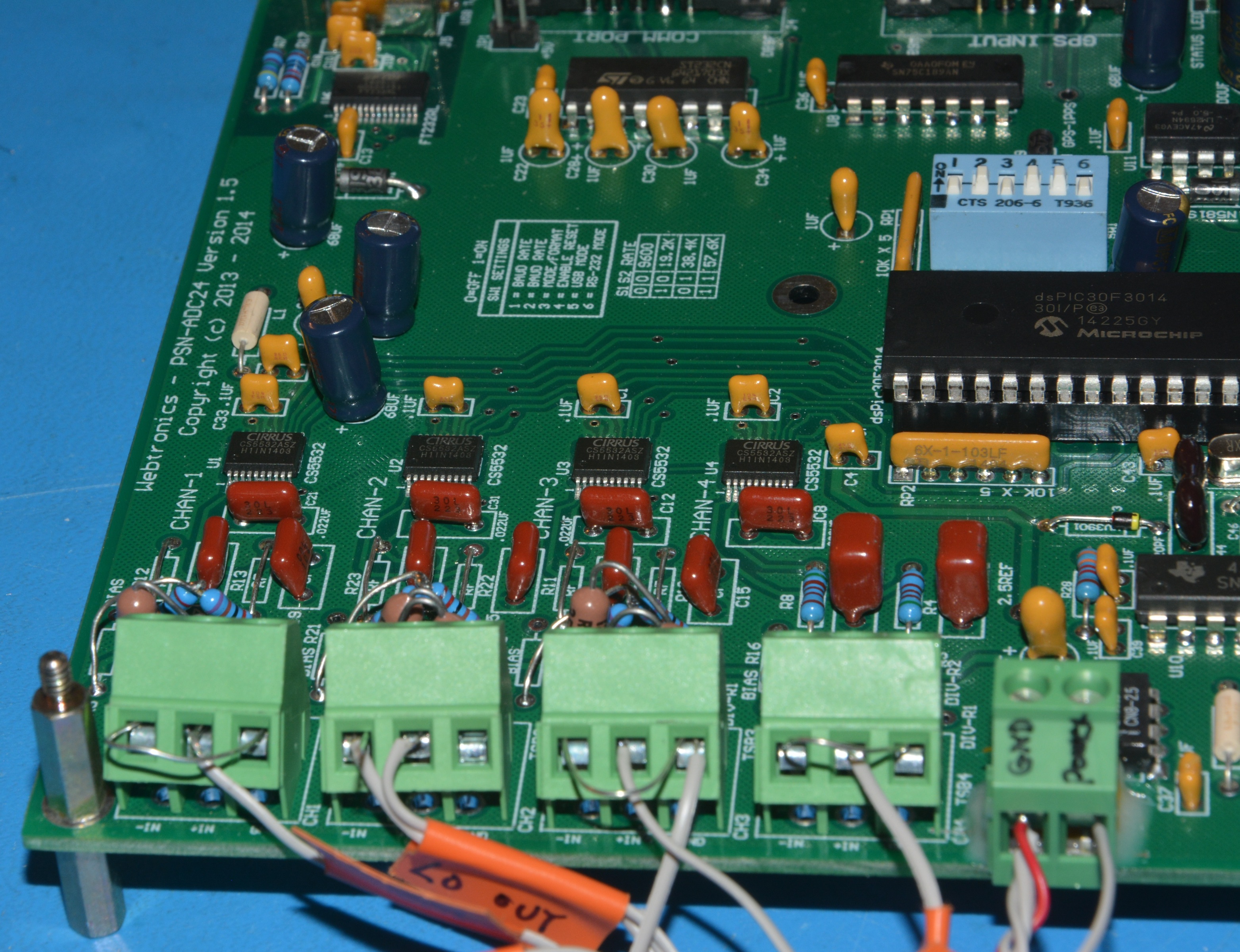
The CS5532 from Cirrus Logic has an internal chopper-stabilized PGA with good noise specs, as low as 6nV/rtHz.
Voltage reference is the 2.5V LT1019CN8-2.5 (3ppm/C stability, 0.05% initial accuracy)
The ADC bipolar full scale range is ±2.5V (-VREF to +VREF) when gain=1. (I'm assuming Larry sets the VFS bit = 1)
On the board, the ADC is biased at
midrange, so AIN inputs are 2.5Vcm +/- 2.5Vdiff: AIN+ = 2.5 + 1.25, AIN- = 2.5 -
1.25
ADC input voltage
|
ADC counts
|
-VREF / gain
|
0x800000 (-8388608)
|
0
|
0
|
VREF / gain
|
0x7FFFFF (8388607)
|
For Channels 1, 2, 3. At gain > 1 the internal PGA is enabled,
reducing input current to 1.2 nA. Therefore gain = 2 mode is used.
Note: in the table below, DIV = 17.0, the resistor divider ratio
ADC Gain
|
ADC bipolar
full scale range
(AIN+ - AIN-)
|
Channel full scale
differential voltage range
(IN+ - IN-) |
ADC counts
|
Quantization
|
WinSDR
'Amp Gain'
Setting
|
1
|
±2.500 V |
±42.5 V |
(IN+ - IN-) / DIV / 2.5 * 2^23
|
5.07 uV / LSB
|
0.0588
|
2
|
±1.250 V |
±21.25 V |
(IN+ - IN-) / DIV / 1.25 * 2^23 |
2.53 uV / LSB
|
0.1176
|
4
|
±625 mV |
±10.625 V |
(IN+ - IN-) / DIV / 0.625 * 2^23 |
1.27 uV / LSB
|
0.2353
|
8
|
±312.5 mV |
±5.313 V |
(IN+ - IN-) / DIV / 0.3125 * 2^23 |
633 nV / LSB
|
0.4706
|
16
|
±156.3 mV |
±2.657 V |
(IN+ - IN-) / DIV / 0.15625 * 2^23 |
317 nV / LSB
|
0.9412
|
32
|
±78.13 mV |
±1.328 V |
(IN+ - IN-) / DIV / 0.078125 * 2^23 |
158 nV /LSB
|
1.882
|
64
|
±39.01 mV |
±664 mV |
(IN+ - IN-) / DIV / 0.0390625 * 2^23 |
79.1 nV / LSB
|
3.765
|
Note: WinSDR doesn't seem to take the
ADC gain setting into account when displaying the data in units of "ADC
volts". So divide by gain to get the correct value. See this spreadsheet for my measurements.
Before connecting to the instrument, I made some noise and frequency
response measurements of the ADC.
The digital filter inside the ADC has a sinc5 rolloff. This means you
need to sample significantly faster than Nyquist to minimize
attenuation of high frequencies. Since I'd like a flat measurement
bandwidth of 20 Hz, I chose to sample at 200 sps, the highest supported
rate in WinSDR. (There are a couple downsides to this: more noise due to less averaging, and the loss of the 60 Hz notch
filter, so AC mains noise might become a problem.) An alternative
would be a digital equalization filter to compensate for the sinc
rolloff, while running at a lower sample rate.
Frequency
|
Measured attenuation
|
1 Hz
|
0 dB
|
2.5 Hz
|
0 dB
|
5 Hz
|
0.04 dB
|
10 Hz
|
0.08 dB
|
20 Hz
|
0.22 dB
|
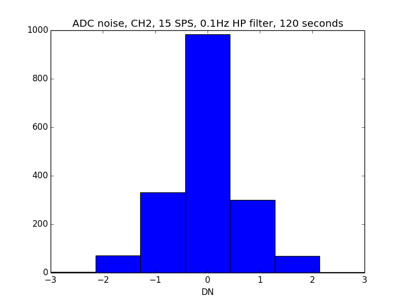
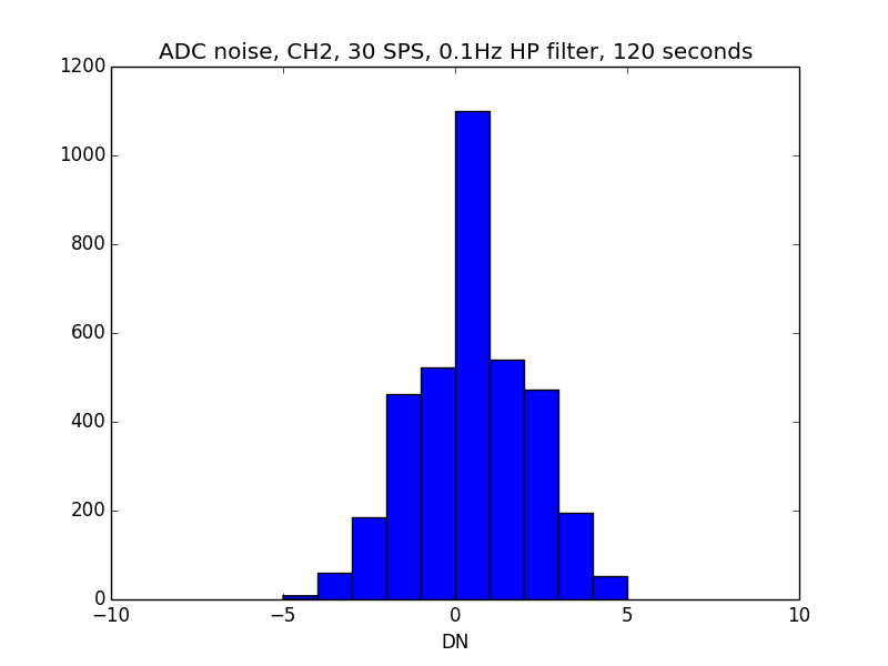
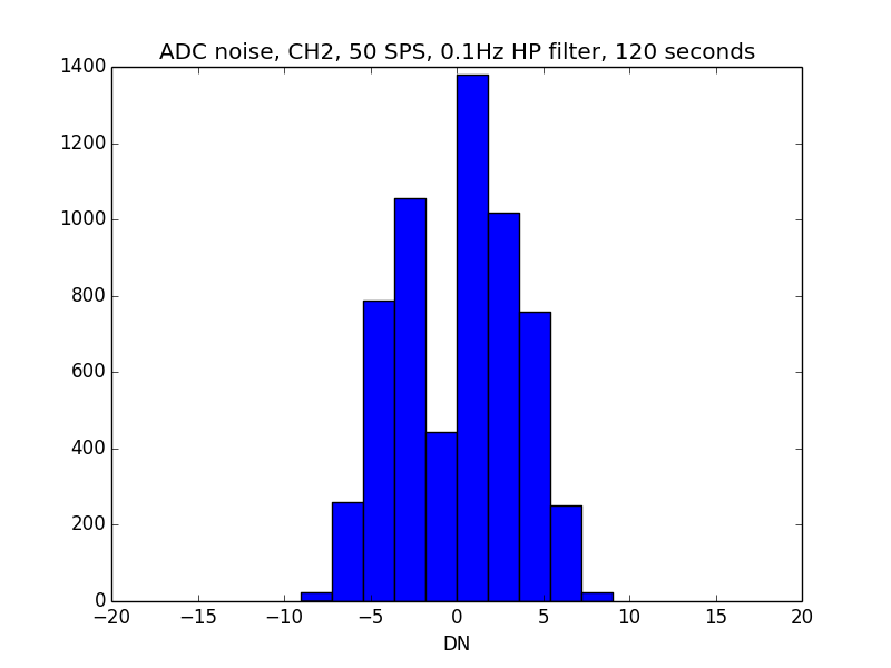
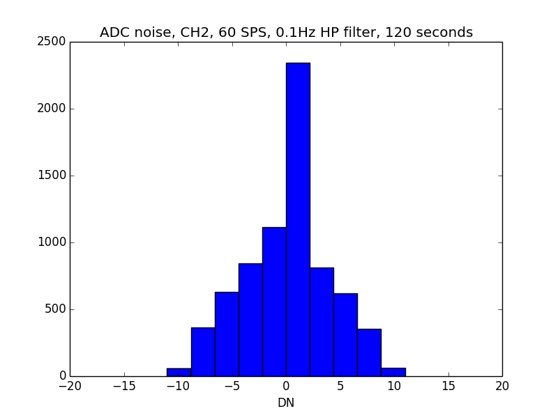
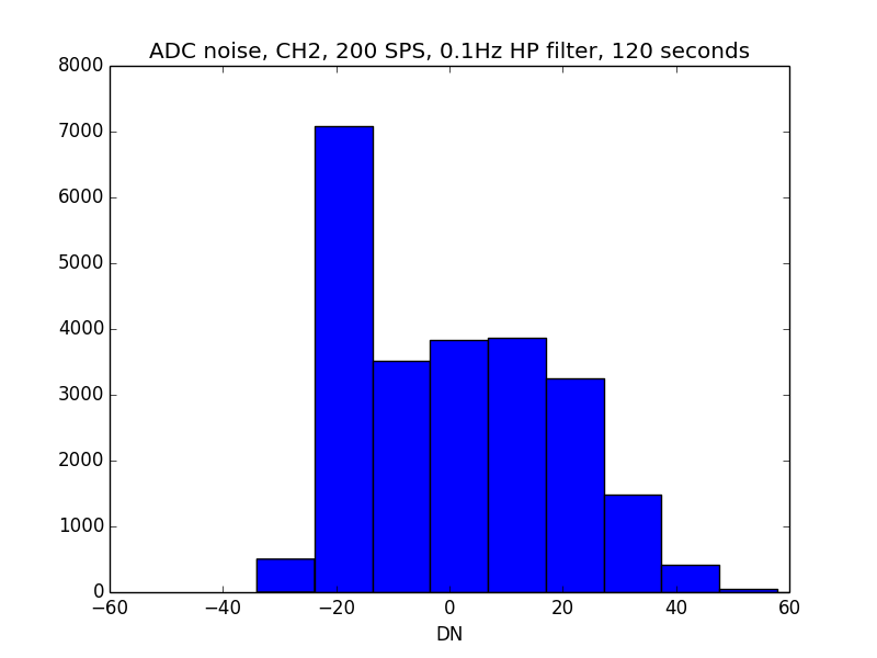
Noise was measured with inputs shorted. These numbers are worse than
the data sheet spec by 1-2 bits. But I don't really trust the
datasheet. There are also some funny noise distributions at 50 and 200 SPS.
Note: noise
free bits = ln(Full-scale range / Vpp noise) / ln(2):
CH4. Divider=1, Gain=1, 0.1 Hz HP 2 pole filter, 120 second window.
Samples / sec
|
DN p-p noise
|
uVpp noise
|
Noise Free bits
|
15
|
9
|
2.7 uVpp
|
20.8
|
30
|
9
|
2.7 uVpp
|
20.8
|
50
|
15
|
4.5 uVpp
|
20.1
|
60
|
16
|
4.7 uVpp
|
20.0
|
200
|
125
|
37 uVpp
|
17.0
|
CH2. Divider=17, Gain=2, 0.1 Hz HP 2 pole filter, 120 second window.
See the "Results" section below for a PSD of the ADC data with inputs shorted, and compared to Yuma-2 outputs.
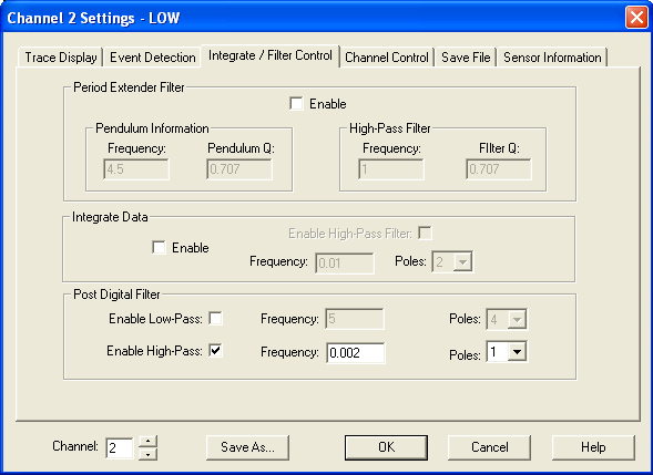
Filtering in WinSDR is an
ongoing experiment for me, but currently I am running only high pass filters on the raw data:
- Low gain channel: 0.002 Hz HP 2 poles
- High gain channel: 0.002 Hz HP 2 poles
In WinQuake I have played with several filtering options, including the
period-extending inverse filter. I still have a lot to learn about best
practices here.
For distant quakes this filter does reasonably well:
- HP 0.002 Hz 1 pole, LP 0.07 Hz 4 pole
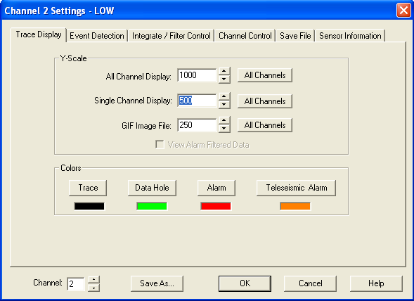
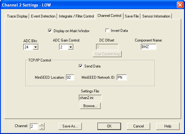
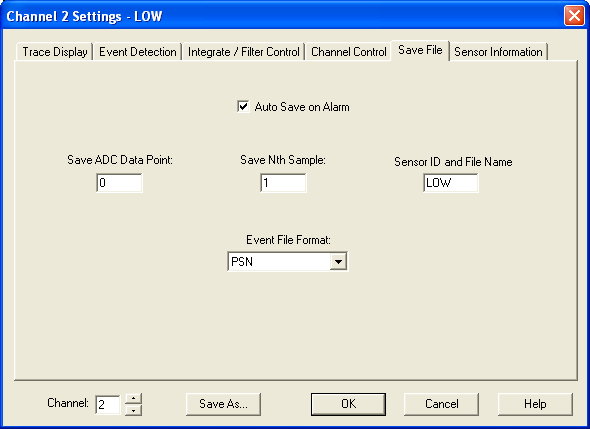
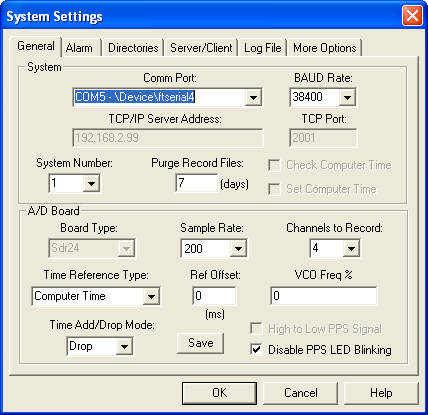
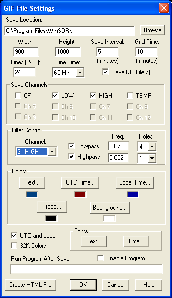
WinSDR Configuration
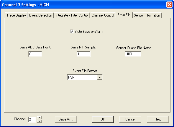
Click on the images below for full size. Configuration of WinSDR, low gain channel:

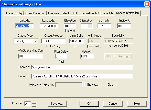
High gain channel:
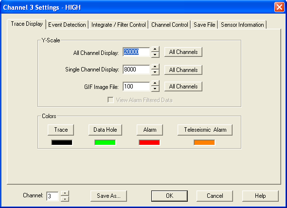
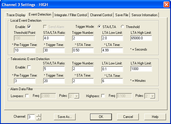

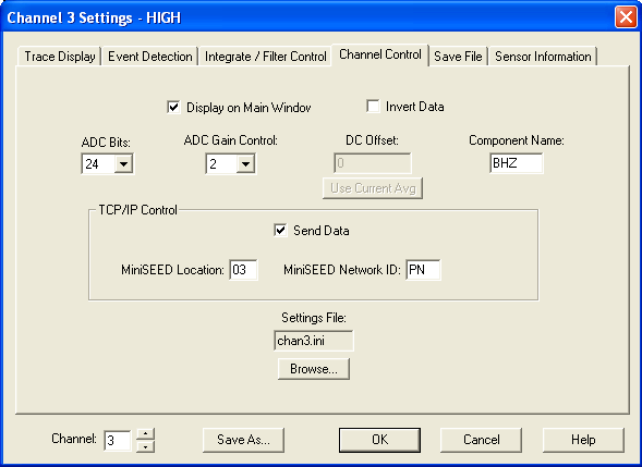

System settings:
Larry has generously provided a utility called drf2txt
that will dump the data from the WinSDR daily record files to plain
text and CSV format for further processing. I find this useful to
further process the data with some python scripts.
WinSDR has a nice feature, a TCP server on port 16064, that can be used
to receive the raw ADC measurements. I'd like to use this to tap
the data stream so I can play around with the live data, without
interrupting the data collection and graphing in WinSDR.
Calibration
To ensure we're making accurate meaurements, it's necessary to make
various measurements so we can properly calibrate the output of the
instrument.
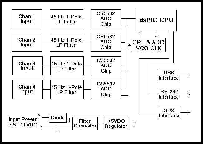
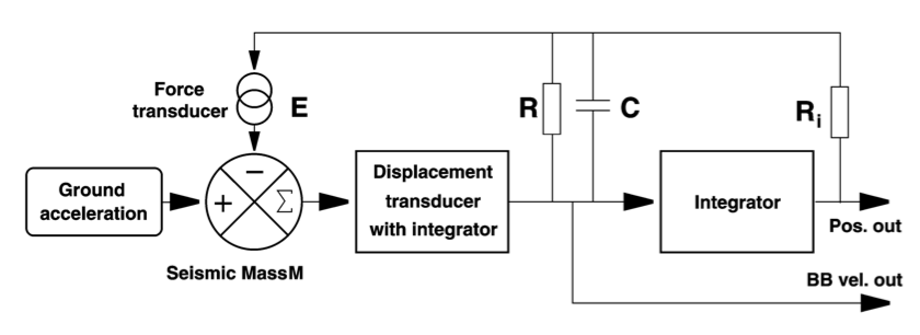
The FBV is a velocity broadband seismometer with this architecture:
The instrument parameters are summarized here. See the sections
below for details on how these were determined. The ADC numbers assume
200 SPS, and gain=2, and no filtering.
| Velocity response |
flat from 0.02 Hz to 30 Hz
|
|
Output channels |
high gain, low gain, internal temperature, and centering force |
|
Coil Forcing Constant, Gn |
9.3 Newtons / Ampere |
Coil / Magnet
|
41.0 ohms, 542 turns 34AWG / N45 magnet |
|
Generator Constant (Ag) |
336.2 Volts / meter / sec |
|
Ag High gain output, (Ag HI) |
33,599 Volts / meter / sec |
|
Ag Low gain output, (Ag LOW diff) |
1,344 Volts / meter / sec |
|
Boom free period |
2.3 seconds
|
|
Boom moment, M0 |
87.5 g
|
|
|
ADC board input impedance
|
38 kOhm
|
|
ADC divider ratio |
17.0
|
|
ADC reference voltage |
2.5V |
ADC input full scale range, gain=2
|
+/- 1.25V (-VREF/2 to +VREF/2), Vcm = 2.5V
|
ADC board full scale range, gain=2
|
+/- 10.625 V (for -VREF/2 to +VREF/2) |
| ADC
Quantization |
2.53 uV/Count (24 bits) |
ADC gain flatness
| -0.2 dB at 20 Hz
|
|
Quantization (HI) |
0.0753 nm/s/count. (unfiltered ADC noise: 9 nm/sec pp) |
|
Quantization (LOW diff) |
1.88 nm/s/count. (unfiltered ADC noise: 225 nm/sec pp)
|
Clipping level (HI)
|
632 um/s
|
|
Clipping level (LOW diff) |
1.58 cm/s
|
Measure critical component values
Measured by U1272A @ 22.2C
Ci
|
30.452 uF |
Cd
|
30.436 uF |
C1
|
not measured. nominally 1 uF |
Ri
|
14.985K |
Rcoil
|
41.0 ohms |
Forcing coil constant Gn
The coil constant, Gn, was measured two ways. Unfortunately there's
some discrepancy in the two results, but I think this is due to my
reconfiguration of the magnet and pole piece, and some slight
misalignments.
First, the magnet/coil assembly was tested separately, by placing magnet assembly on a scale,
suspending the coil above from an aluminum bar. Inject known current (+/-50mA) into
coil and measure change in weight.
Gn = Δ Weight * 9.81 / current
Less than +/- 3mA, coil constant: 10.5 +/- 1.0 N/A
From +/- 50 mA, coil constant: 9.62 +/- 0.48 N/A.
(These values had been measured with a slight misalignment of the coil.)
542 turns, AWG34, N45 magnet, Rc=43.7 ohms.
Gn = 9.6 +/- 0.5 N/A
GN can be measured with the
instrument assembled and operating normally. First record the coil
resistance, Rc, and the measured value of Ri. Attach an accurate
voltmeter to the"CENT FORCE" output, pin 6, and turn on the
seismometer. Balance the boom if necessary and after it stabilizes,
record the voltage, VCF . Then place a 500mg weight on the top of the
boom at the same distance from the pivot as the center of the coil. If
necessary, any approximately 500mg non-magnetic object whose weight is
accurately known, such as a #6 brass washer, may be used instead of a
500mg standard weight. After the output on pin 6 settles, record the
new voltage. The coil constant Gn = W/ δVCF * 0.00981*
(Ri+Rc) N/A, where W is the test weight value in
grams..
Using the second method, on a fully assembled instrument, remeasure Gn by using CF output and known mass on boom, at coil mount:
Ri = 14.985K. Rc = 41.0 ohms.
Measured CF = -0.5622 V
Add 500mg calibration weight. Allow to stabilize 5 minus. CF= -8.513V
delta V = 7.9508 V
delta I = 7.9508 V / (14985+41 ohms) = 5.2914e-4 Amps
delta F = 500e-3/1000 * 9.81 = 4.905e-3 N
Gn = F / I = 4.905e-3 N / 5.2914e-4 A
Gn = 9.27 N/A
Boom mass M0, M1
First, the instrument may be
assembled without the spring and the effective boom weight measured by
means of a sensitive scale, arranged to support the beam so that it is
level, at a point which is the same distance from the pivot as the
center of the coil/magnet. That gives M0. When using particularly
flexible (Kapton) flexures, watch to be sure that without the spring,
they aren't flexing downward too much during the measurement.
Spring: 4.7g
Boom w/o spring or weights (including vertical brass threaded rod): 165.1g
Boom with weights: 210.3g
Hanging support: 10.5g + 0.5g nut = 11.0 g
Measured weight at nominal position: 98.5g
Net boom mass, M0 = 87.5g
M1 is difficult to measure. Estimated 110 g
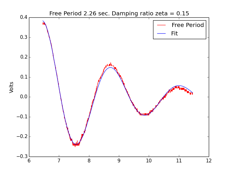
Free period
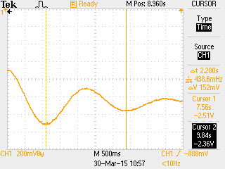
Free period was measured by disconnecting the coil, selecting
GAIN=1 by
removing JP1, and measuring POSN_ERR output while generating an impulse
with a canner air duster. This was repeated several times. The
measurement was made 7.5 seconds after the impulse to try to capture
the small signal reponse. Period was measured on the scope to be 2.3
+/- 0.1 sec. An FFT of the data indicated a period of 2.26 sec. Zeta
was determined to be 0.15, by fitting the data to a damped harmonic
oscillator.
Sensor gain, Rsensor
To measure the sensor gain, remove
jumpers JP1 and JP2 and unplug the connection to the forcing coil.
Arrange for the boom to seek its upper stop, either by installing and
adjusting the spring or by means of an external spring such as a rubber
band gently lifting the boom. Mount a micrometer or micrometer head to
press down on the boom at the same distance from the pivot as the
center of the coil. Mount the micrometer so that it can move the boom
over its vertical range. Starting with the boom approximately centered,
connect a meter to the 'POS ERR' output, pin 7 and turn on the
electronics. After the voltage stabilizes, using the micrometer, move
the boom in steps in both directions from center over about half its
range, approximately ±0.4mm or ±0.015", while recording the micrometer
readings and corresponding output voltages. The slope of the data curve
at its zero-volt point (change in voltage/change in position in mm)
should be approximately 12.5V/mm, which, multiplied by R6/R29
(nominally 1/10), will give the value of rsensor
Since I didn't have a micrometer head, I chose to do
this measurement
on my mill. Rubber bands provided upward tension on the boom. A pointed
tip in the chuck pressed down on the boom at the coil mount screw. The
Z-axis DRO measured position as I recorded POSN_ERR output voltage.
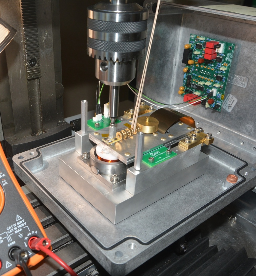
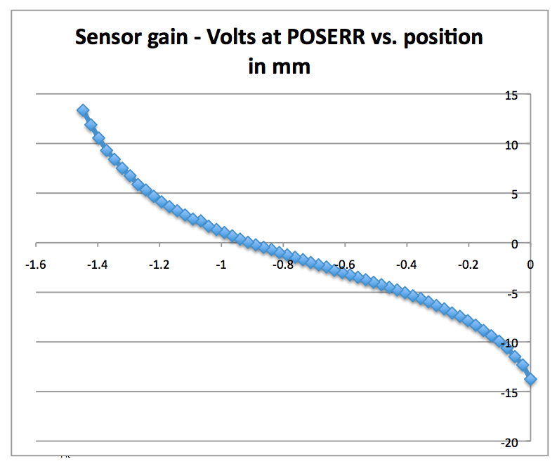
Notice how the zero crossing is not in the symmetrical part of the
curve. I suspect the boom is not planar with the PCB at zero position,
possibly due to flexture sag or machining errors. The flexture
gap was set to 10 mil with a feeler gauge. Accounting for the -10X gain
of the POSN_ERR output stage:
Rsensor: 1118 V/m
Centering Force
The centering force output was measured
to be delta -7.951V with an additional 500 mg calibration weight on the
boom, at the coil mount point.
CF = -7.9508/500e-6 = 15902 V/kg
Centering Force sensitivity = -15.9 Volt / gram, where negative means additional force supplied by the coil.
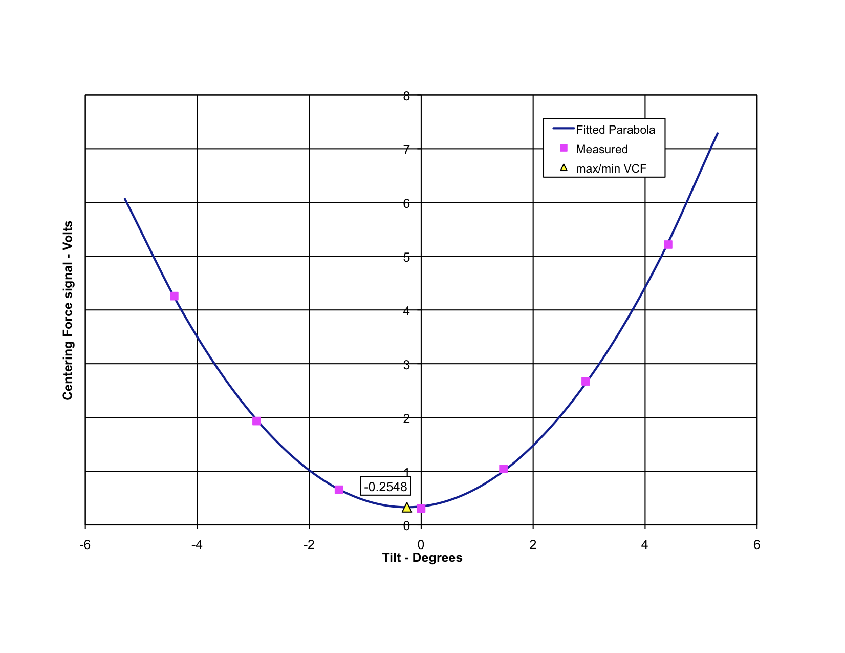
Balancing
You really can use two balance
weights, one horizontal and one vertical, though just one can be used
if you accept a somewhat more complicated adjustment procedure. A
properly balanced boom will have its center of mass lying in the same
plane as the pivots. This means that its sensitivity to
horizontal motion is minimized; or stated another way, its sensitive
axis is close to vertical.
Then the boom mass and the horizontal location of its COM will need to
balance the spring when its length has been adjusted to get 3-seconds
or so, free period. The spring adjustment sets the free period;
the mass is just trimmed horizontally for balance.
If you used two balance weights, you could make them adjust the x and y
coordinates of the COM somewhat independently.
Initially the COM will be located below the level of the pivots, mainly
because the coil mass is fairly significant and is below the pivot
plane. To balance, with the spring removed, but everything else on the
boom in place, hang the boom coil down. If the pivot gap isn't
too much over 0.010", the flexures should work fine in
compression. The vertical trim weights are adjusted until the
boom hangs straight down. Horizontal balancing is done at the time you
are first adjusting the free period. Fine trimming can be done
with a thumb nut or two on an horizontal brass screw, mounted as you
observed below. With minimal horizontal trim weight, start
shortening the spring until the boom balances and check the oscillation
period. It will be less than 3 sec. Shorten the spring by a
couple of
thousandths (of an inch), temporarily add a bit of weight near the coil
for balance (small brass washer or nut?), and check the period.
Shorten more and rebalance, etc., etc. When you get up to
something around 3 seconds, you can permanently attach equivalent
weights (on the coil screw?) and then make final balance adjustments
with the horizontal thumb screw(s).
Download the balancing spreadsheet:
Tilt_test_357.xls
The vertical axis of the instrument is aligned within 0.26 deg of true.
Horizontal sensitivity is 0.44% of vertical sensitivity. This is a
pretty good result.
Since the sensitivity angle is negative, the vertical trim weight is slightly too low.
The centering force error is -22 milligrams, so the horizontal trim weight is slightly too close to the pivot.
Confirmed polarity of coil matches schematic - positive
voltage moves boom upwards. The loop polarity spreadsheet has been recently updated to account for the Yuma2 circuitry.
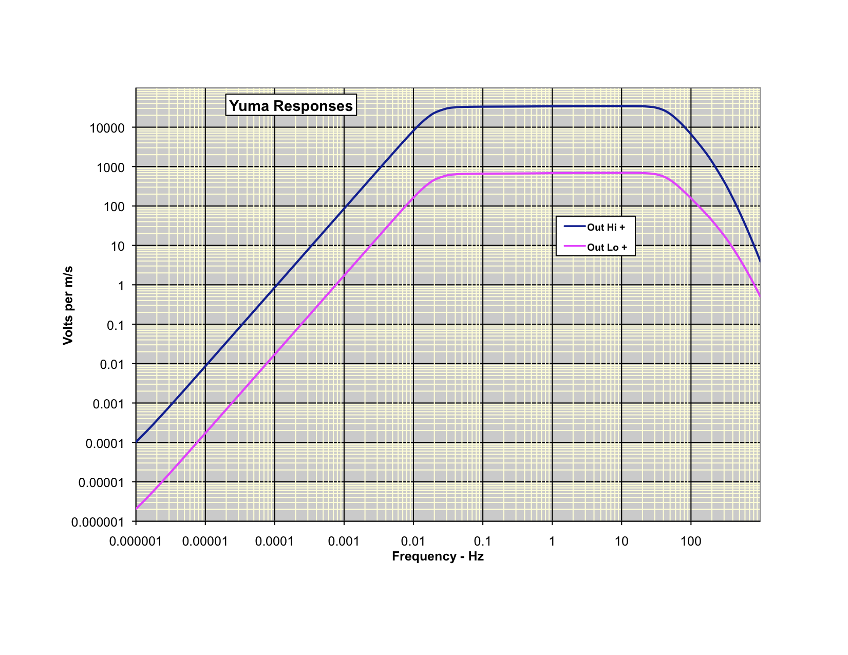
Instrument Generator Constants
Computed from Loop8Y.xls:
| Ag |
336.20 V/m/s |
At feedback Loop output
|
| A hi + |
33,599 V/m/s |
OUT HI +
|
| A low + |
671.98 V/m/s |
OUT LOW + |
| A low - |
-671.98 V/m/s |
OUT LOW - |
| A low (total) |
1,344 V/m/s |
(Out LOW +) - (OUT LOW -)
|
As you can see later, this matches the SPICE simulation within 2%.
Poles and zeros
Transfer function computation, using Loop8Y:
Poles:
S-domain
|
Corner Frequency
|
Channel
|
|
-8.433e-4 +/- 0.08498 |
0.02 Hz
|
both
|
-209.7 (appx)
| 33.4 Hz
| both
|
|
-1000 + 0j |
159 Hz
|
both
|
|
-1002632 + 0j |
160 KHz
|
LO -
|
-1002632 + 0j
|
160 KHz
|
LO +
|
-100263 + 0j
|
16.0 KHz
|
HI
|
Note: The pole at 33.4 Hz is estimated based on LTSpice simulation.
Zeros:
S-domain
|
Corner Frequency
|
Channel
|
|
0 + 0j |
0 Hz
|
both
|
|
-4.167e-6 + 0j |
0.7 uHz
|
both
|
The instrument response to ground velocity is calculated using Brett's
Loop8Y.xls
spreadsheet, using measured values for electrical and mechanical
parameters, and the Rev 4.0 schematic. M1 has been estimated at 155 g.

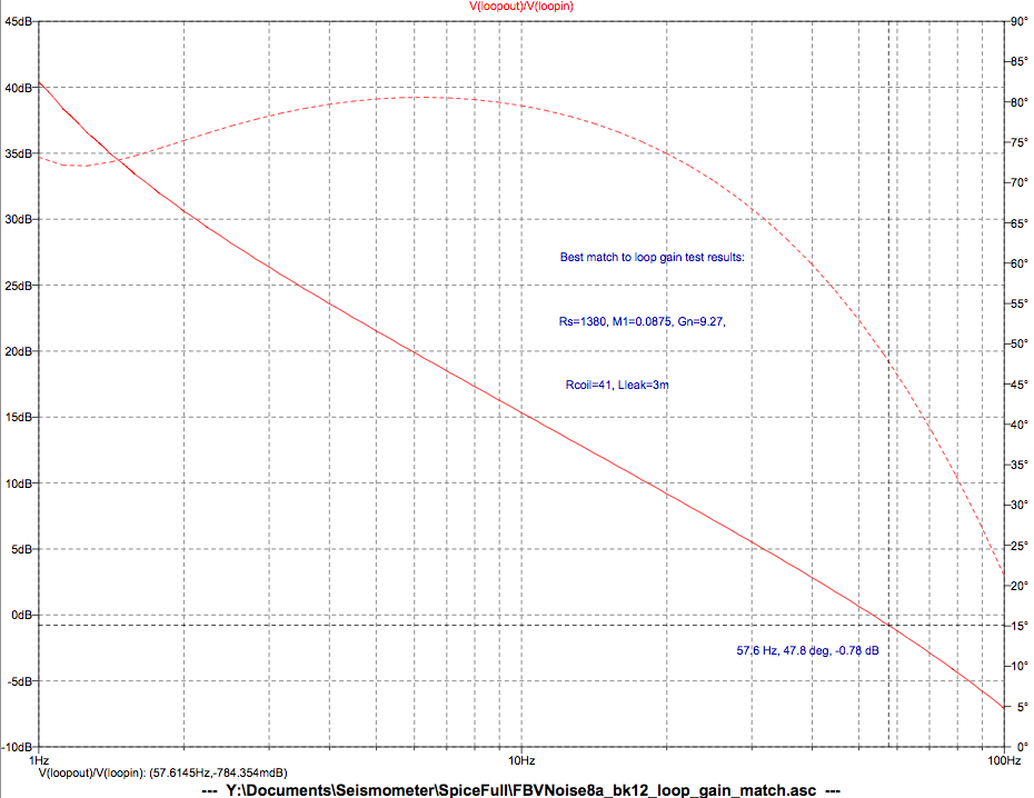
Loop gain measurements
Using the
loop test board,
I measured the gain and phase of the feedback loop. The loop was
broken and a signal generator was inserted to inject a signal into the
fedback loop. By
measuring voltage and phase shift,
several things about the feedback loop are characterized. The crossover
frequency, where loop gain drops to unity, and phase margin at the
crossover frequency are important metrics to assess loop stability and
compare against expected values.
Surprisingly, the crossover frequency was much higher than
expected. It was measured at 58 Hz, with 48 degrees phase margin.
This is sufficient for stability, but a crossover frequency closer to
30 Hz was expected based on the Loop8 spreadsheet.
I ran some Spice simulations to investigate the discrepancy. See the Simulation section below for details.
Over 5 days, the Centering Force output (inverted), was compared
against the internal temperature sensor, over a narrow range of
temperatures. The sensor is
mounted on the PCB, while the CF is primarily affected by the
temperature of the spring. CF is a -1X output from the integrator, so
the integrator has a +31 mV / C coefficient. This is exactly one tenth
the value measured by another builder. I'm not sure what the source of
this discrepancy is.
Using the coil force constant, and the value of Ri, this represents a
force difference of 2 mg / C. Using M0 measured above, this is
23.1 ppm / C.
dF/dt = 0.267 V/degC / 14985 ohms * 9.6 N/A / (0.0875 kg * 9.81m/s^2) * 1e6 =
206 ppm/degC
The spring constant is expected be about 250ppm/C.
(On the plot there is an inadvertent gap of several hours when the data recording was interrupted.)
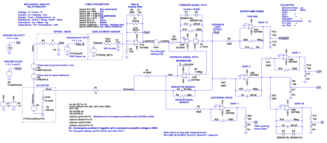
Simulation
Starting with Brett's SPICE model of the mechanicals and control loop,
I added the output amplifiers of the circuit and tweaked the
parameters to match my Yuma, as measured. SPICE is typically used
as an electrical simulation tool, but mechanical systems can be modeled
as well, since they share the same underlying physical equations.
In this case the spring-mass-damper and forcing coil were modeled using
the 'Force-Voltage' analogy for translational mechanical systems.
In SI units:
Force (N) = Voltage (Volts)
Velocity (m/s) = Current (Amps)
Mass (Kg) = Inductance (Henries)
Damping (N/m/s) = Resistance (Ohms)
Compliance (m/N) = Capacitance (Farads)
Displacement (m) = Charge (Coulombs)
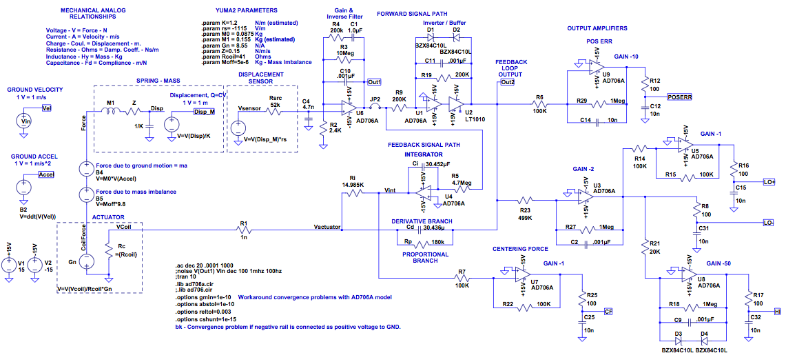
If you want to simulate in LTSpice, here's the schematic file and the AD706 model.
It's nice to have a complete model of the electromechanical system that
be be simulated in its entirety. A few comments about the model:
Displacement sensor is assumed to be linear.
Spring TempCo not included.
Simulations tested: transient, AC, noise.
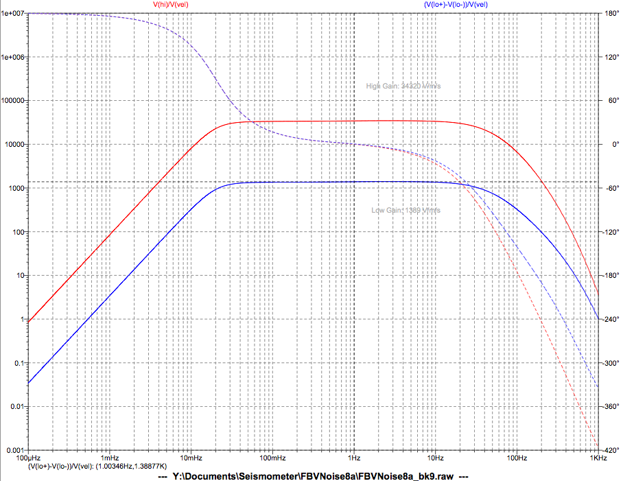
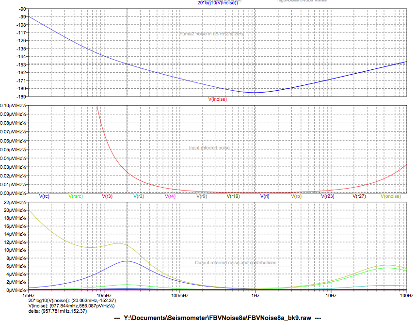
Simulation results match the Loop8 spreadsheet closely. Low gain channel
is determined to be 1389 V/m/s. High gain channel is 34320 V/m/s. This
is within about 2% agreement. Simulation predicts flat velocity
response from 21 mHz to 33 Hz. Noise at 20 mHz is predicted to be
-153 dB m2/s2/Hz. At that frequency, the
largest contribution to noise is the Johnson noise of the coil
resistance (7 uV/√Hz, referred to output.)
The coil noise is still the subject of some uncertainty. It appears the
real instrument has lower noise than the simulations suggest. Brett is
using a custom op-amp noise model that has noise more closely
resembling real measurements, at or below the NLNM noise floor.
The AD706 macro-model simulates worst case datasheet parameters, but
for noise the datasheet only provides typical values.
To investigate the discrepancies found during loop gain testing, I
tried a few things to try to make the Spice simulation fit the measured
data.
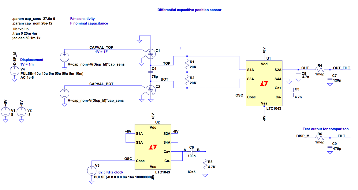
I made a separate circuit model to simulate the position sensor in
isolation.
The original Yuma spice circuit had a pole in the position sensor
circuit that was slightly off, compared to the simulation results of
the LTC1043 circuit. This affected the phase margin of the loop.
The LTC1043 is a switched capacitor circuit and
the model from Linear does not seem to be capable of AC analysis. So I
ran a transient analysis and fit the step response of the circuit to a
single-pole RC filter. I used a voltage-variable capacitor model from here.
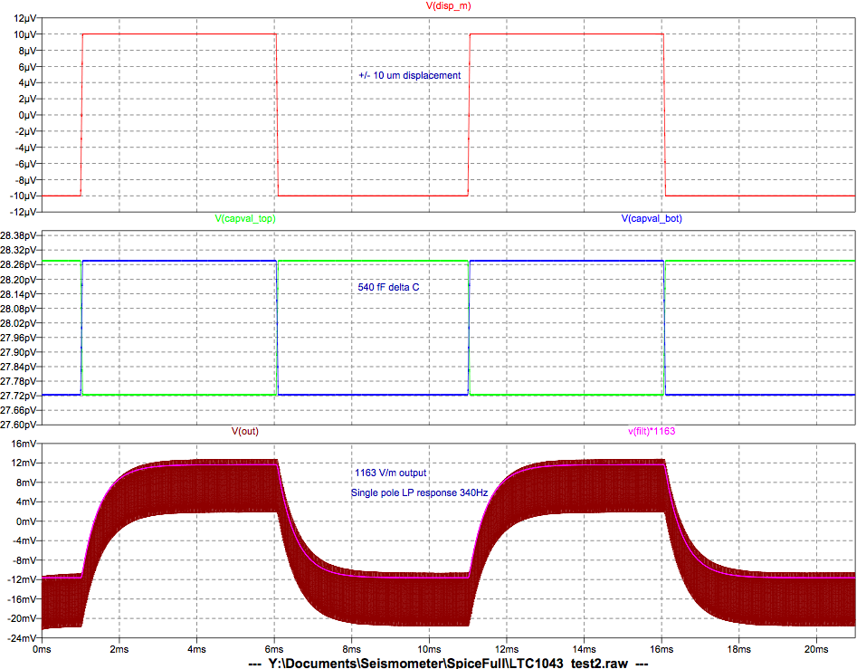
The result was a response with a single pole at ~340 Hz. The
sensitivity of this circuit is quite amazing. For a +/- 10 micron
displacement, it is measuring only half a picofarad of capacitance
change! And typical boom movements are much less than that.
LTSpice schematic and capacitor library and symbol.
Next, I played
with the M1 mass to shift the crossover frequency to the right place
(decreased it to M0 value). I played around with the leakage
inductance of the coil to get
the right shape to the gain curve near 100 Hz. I adjusted the Rsensor
gain to correct the overall gain (increased it by 24%). After this, I
had a circuit model that
matched the measured data more closely. But I have some doubt
whether these adjustments reflect reality. They don't agree with my
earlier measurements of the sensor gain, and the mass change doesn't
make sense to me.
Closest match was found to be: Rsensor = 1380 V/m, M1 = 87.5g, Gn=9.27
N/A, leakage inductance = 3 mH. At Fc=58 Hz, the gain of the
simulated circuit is -0.8 dB, and the phase margin is 48 deg.
LTSpice schematic.
Installation
As mentioned earlier, care must be taken to install the instrument
properly for best results. Based on recommendations by Brett, Dave, and
other members on the mailing list, I've chosen a few things for my
particular situation. Living in town, in the Bay Area, I do not have a
low background-noise site. Traffic, trains, low-flying aircraft,
neighbors, and household equipment all contribute significant seismic noise, which this instrument easily picks up.
Currently my Yuma is set on a granite tile, which is resting on the
concrete floor of my garage. The legs are leveled, based on earlier
calibration. Small pieces of lead sheet are placed under the legs, and
at three points between the granite and concrete to help stabilize the
instrument and reduce noise from differential CTE of materials.
The instrument is connected to the ADC with a ribbon cable of
approximately 18 inches. The cable is currently unshielded, but the
adjacent grounds of the connector pinout provide some minor level of
shielding. The cable is strain-relieved by wrapping it under the Yuma
to avoid pulling on the side of the case.
An insulation wrap made from several layers of polar-fleece fabric
surrounds the Hammond case, with cutouts for the legs. A thick
styrafoam cooler,
without the lid, is set upside down over the installation. A small
weight on top keeps it secure. A future addition might be styrafoam
insulation for the the ADC
case, to keep any temperature-related drift to a minimum.
The ADC is connected over USB to a Raspberry Pi, running ser2net, a TCP/IP to serial port utility that supports RFC2217 for low-level remote control of the port. (See config here.) The Pi is connected over wired Ethernet to the home LAN, and a laptop is running WinSDR. I'm currently using Serial Port Redirector
by Fabulatech to fake a local COM port for this remote setup. I might
change to a freeware alternative, but so far none have proven reliable.
Results
So, the big question is: how well does it work??
Bear in mind that I still have a lot to learn about proper filtering,
installation optimizations, and noise mitigation techniques. But the
results so far have been an eye-opening experience.
The first thing to note is the strong diurnal signature of cultural
noise, all the man-made background that comes with living in a
metropolitan area. My location is 2 blocks from the main throughfare in
town, 1/3 mile to a commuter rail line, and 3/4 mile to the nearest
expressway. Clearly this is not the ideal location for a seismic monitoring
site. Even so, I have to say I'm pleasantly surprised with the
results.
In the Bay Area, small quakes are commonplace. Typically, we've been
getting several per day less than M3.0 within 100 miles radius of my
location. A normal person would likely never feel any of these. These
small quakes are completely normal for the geology of the area. The
Yuma picks these up easily, and depending on their strength and
location they can be quite prominent in the data, or visible only after
close examination.
Large distant quakes, called teleseismic events, are also within reach
of the Yuma. Wikipedia states that modern (professional) seismic
instruments can detect an M5.3 anywhere in the world. Having just
started out with this, I'm just beginning to build up my dataset of
distant quakes. However, a few days after installing the
Yuma, I detected a very clear signature of a M6.2 event over 6000 miles
away near the coast of Chile.
(Note that I had not properly calibrated the WinSDR settings so you can
disregard the y-axis units. I am also just guessing at the locations of
the P and S waves, but they are consistent with a quake at the
specified distance.)
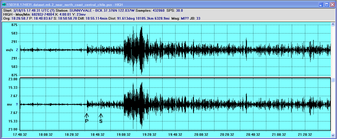
Compare this to the same quake recorded at a college station in central CA:

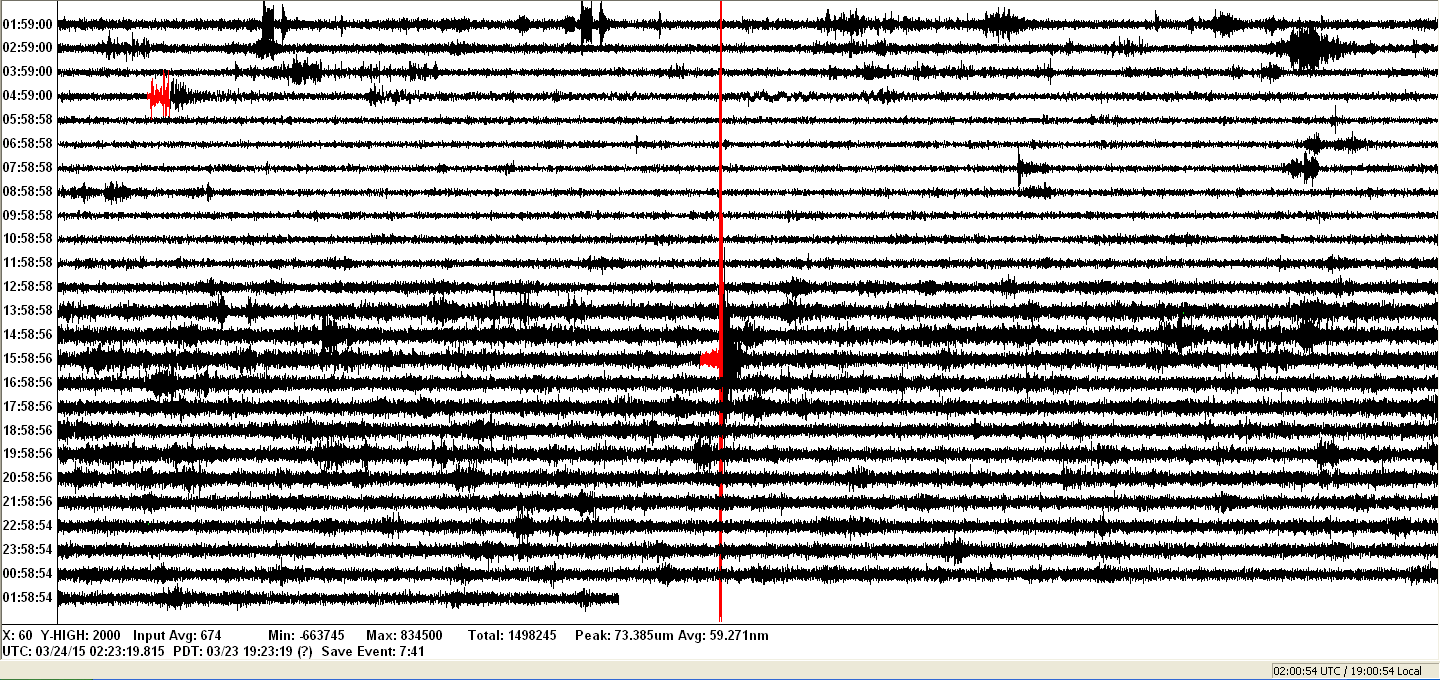
A few days later, a nearby M2.9 occured a few miles away in the
foothills near Cupertino. The strong signature is visible near the
center of the chart. Also on this chart is an M2.7 at 15:47 UTC
and an M2.1 at 08:41 UTC. The rest is mostly local noise.
Notice how the night (top) is much quieter than the day (bottom).
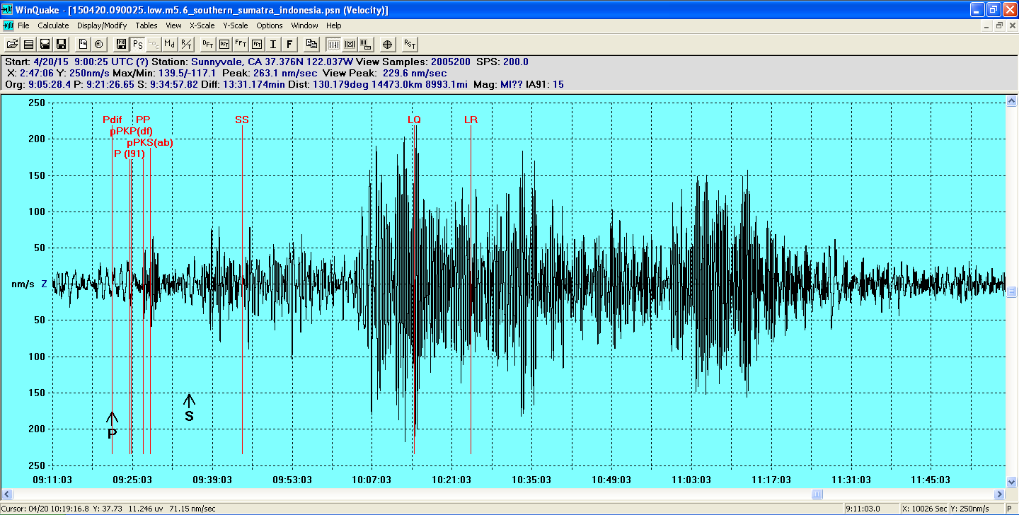
The farthest and faintest I've caught yet was a M5.6 South of Sumatra,
about 9000 miles away. If my calibration factors are to be trusted, the
measured motion was less than 250 nm/sec. This quake arrived at
nighttime when it was quiet. (The markers for LQ and LR are inaccurate
due to the wide variability in the speed of propagation of surface
waves.)
The damaging M7.8 in Nepal, including some aftershocks, came rumbing through over 3 hours.
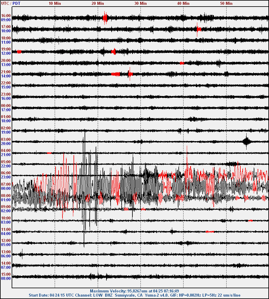
Listen to the Nepal quake as a WAV file,
filtered 0.01 Hz to 0.07 Hz and sped up many times. One second of
audio time is just over 1 hour of real time.
Here are a few distant quakes:
23:54 M5.1 in New Guinea
02:55 M4.7 in Alaska
09:08 M4.7 in Guatelama
10:30 M5.5 in New Guinea
Update 12/30/15: Here are animations of about 6 months of recordings from the low gain channel and high gain channel.
A good quake tracking site is http://earthquaketrack.com/recent
Interesting man-made sources that appear regularly are late-night freight trains, nighttime street
sweepers, and large aircraft on
approach to Moffett Field. There are a few more that I haven't
identified yet. The trains are interesting because I can see them make
their way up or down the penninsula by comparing my traces to those of
another Yuma in Palo Alto, 9 miles away, run by Gary Lindgren. Larry Cochrane has seismometers running in Redwood City, about 15 miles from here.
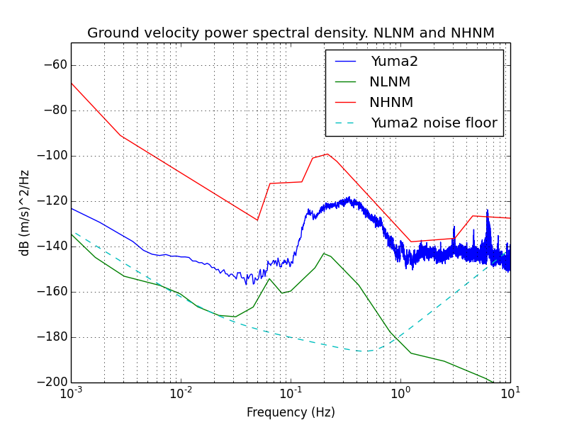
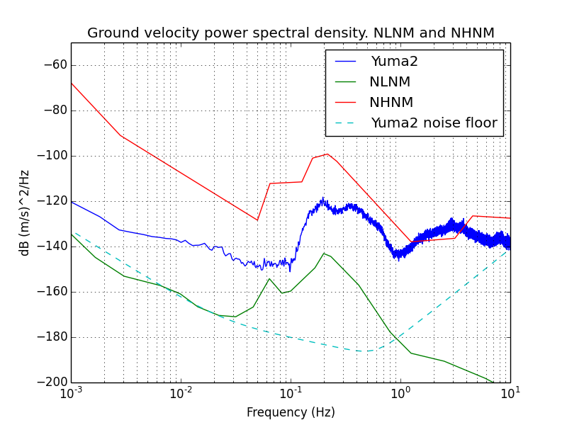
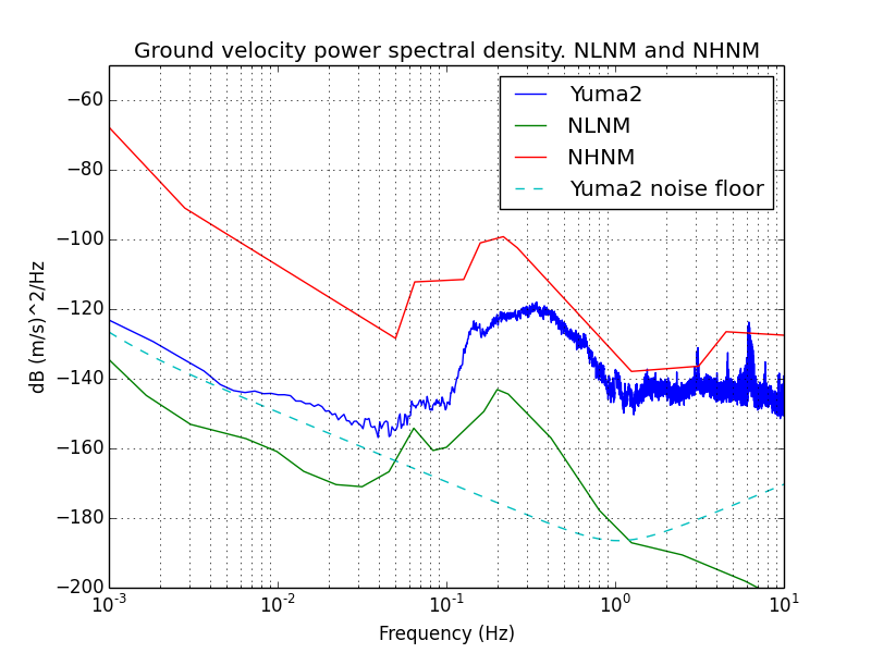
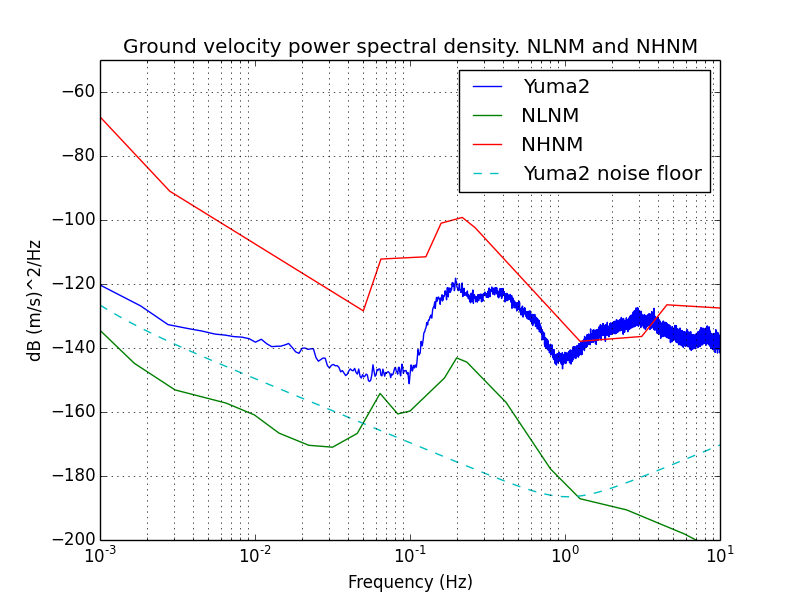
A
power spectral density plot compares the
Yuma low gain output against the
NLNM (New Low Noise Model) and NHNM (New High Noise Model) ground
velocity. These represent worldwide background averages at professional
stations. Each plot represents 7 hours worth of data at 30 sps. The
data was not filtered. First plot is 7 hour of data at night, second is
7 hours of data during the day.
The shape of the data indicates that my Yuma really is picking up
signals consistent with the natural background seismicity of the Earth.
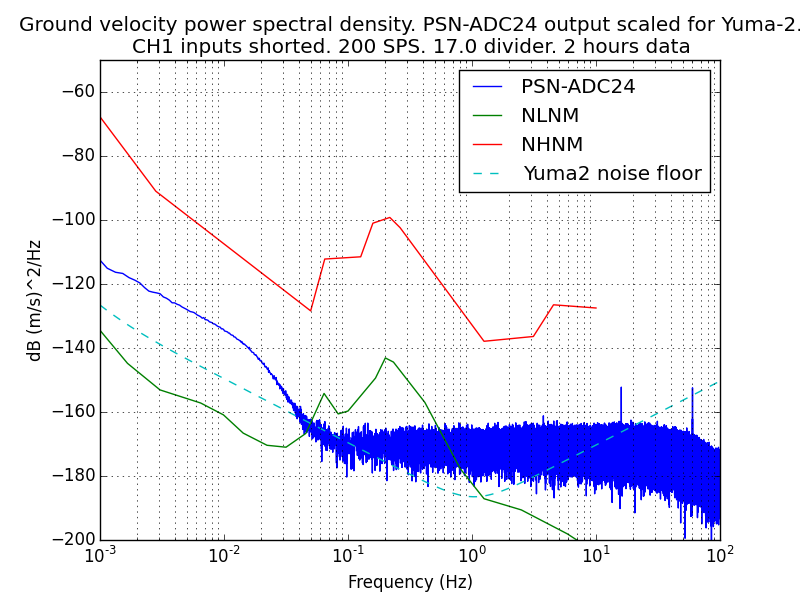
In the plots below, the noise floor was calculated using a SPICE
simulation of the actual circuitry (including Analog's model for the AD706).
I noticed that my noise floor measurements are different from what
Brett computed, using his own custom noise model for the AD706, and
slightly different component values from my Yuma.
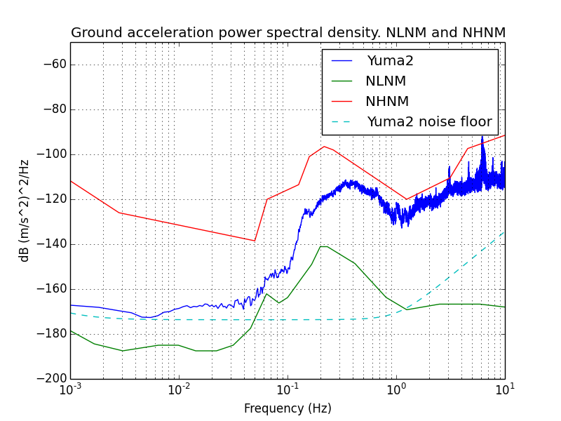
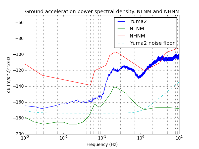
As a comparison, here is the noise spectrum with the ADC inputs
shorted. This was taken over a shorter time period, so the low
frequencies are less accurate:
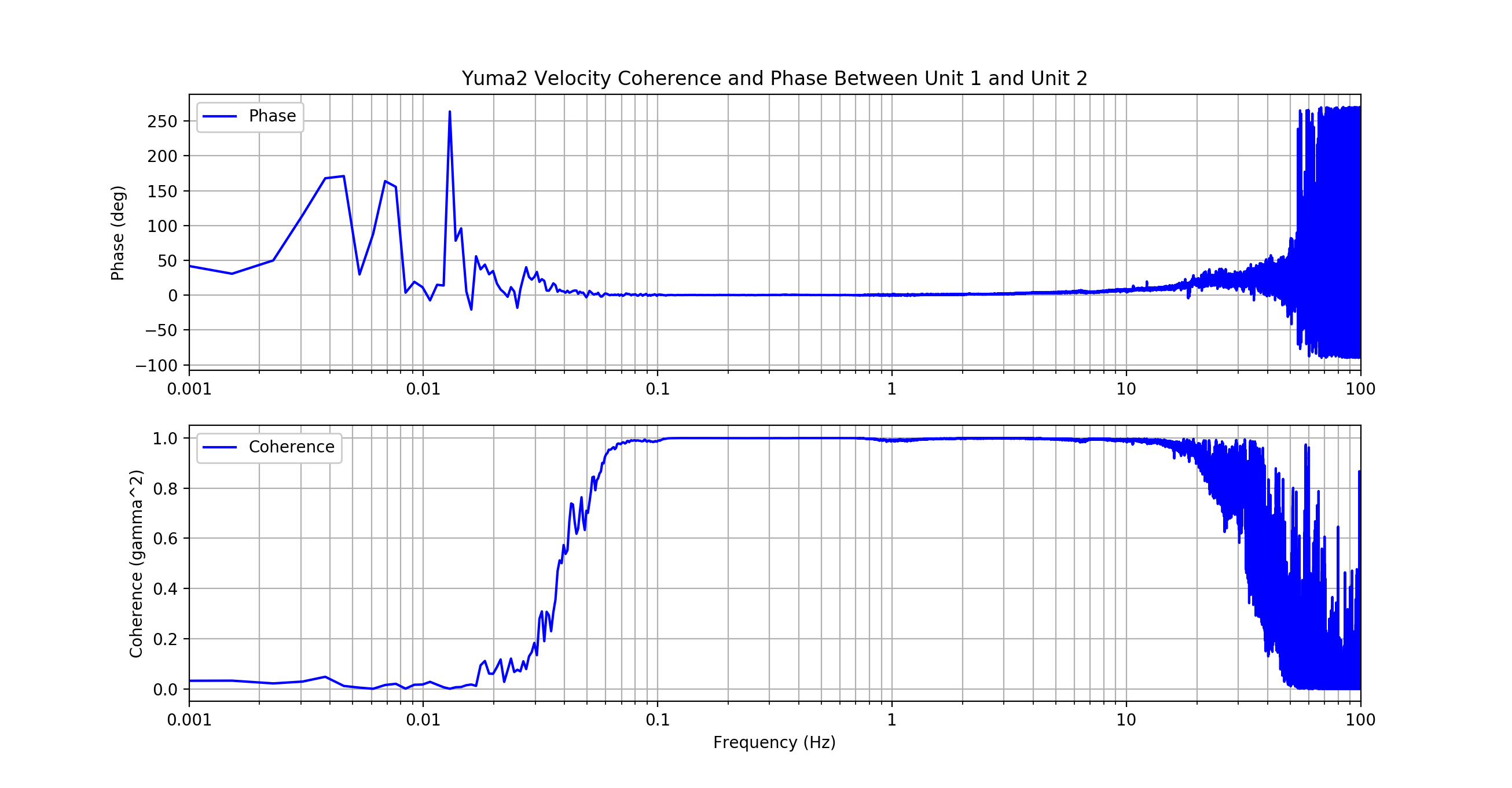
Update 11/20/17: I should have included these coherence plots two years ago when I created them, but better late than never... The two-instrument
Holcomb technique is a way to estimate instrument self noise, by comparing the signal received by two more-or-less identical instruments in the same location. (An even better technique is
Sleeman self-noise measurement,which uses three instruments.)
Using Gary Oliaro's work as a guide, I wrote this python script to generate these plots, which estimate the coherence and self noise from my two Yumas.
The dataset (122615_000000.txt) was taken during a 24 hour period that was relatively quiet, with no major earthquakes and only one small one. Since it was the Christmas holiday, only a single train was passing through. The data was collected with a 0.002 Hz single pole HP filter.
At this time, Unit 2 had an incorrectly-wound coil (too many windings) with a higher force constant, so its gain is lower. Unit 2 was (unfortunately) installed 90 degrees rotated to Unit 1. For this reason they might have had different sensitivities to low-frequency ground tilt. Any horizontal axis sensitivity would have also degraded coherence.
The good coherence (gamma^2 = 1.0) across the range of 0.07 Hz to 20 Hz shows the region where the two instruments produced nearly identical outputs. From this, we infer a low contribution of instrument self-noise in this range.
In the frequency ranges where the coherence drops off, the instrument self noise is larger. The shape of the coherence plot is partly an artifact of the dataset I chose.
During this time there was very little energy measured in the lowest frequency range. When re-running this script against data with several large distant earthquakes, the coherence was much better across all frequencies.
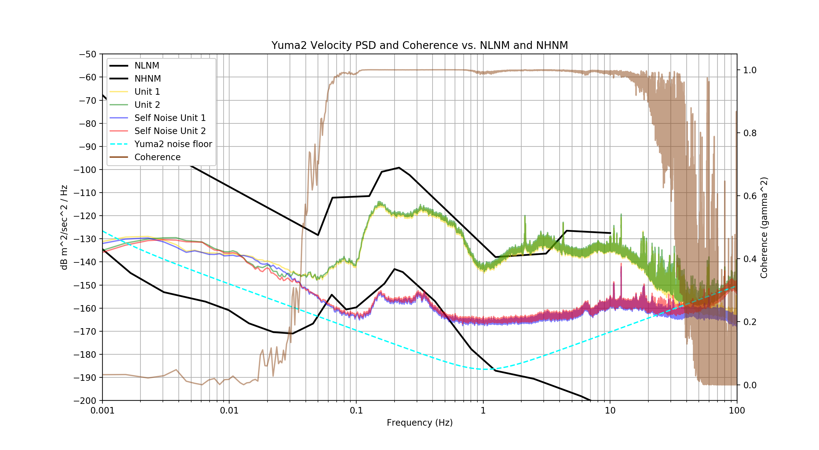
It's also interesting to note the phase difference between the two units. I suspect some of the phase shift from 1-20 Hz could be due to the differences in the coils. In addition to their different force constants, Unit 2 has a significantly higher inductance.
In my Spice simulations, the coil leakage inductance had an notable effect on phase margin of the loop.
Others
Other seismomenter builders are doing exciting things with their instruments. Gary Oliaro has some fascinating pages
about his work using Yuma to measure solid-earth tidal effects. See the
moon pulling on Princeton, New Jersey. Also, check out his detection of earth normal modes
using two Yumas operating coherently.
Larry Cochrane has a nice live page that automatically updates, showing earthquakes from around the world captured using his equipment.
Other local builders have their live Yuma seismometer data online, including Peter Rowe in Los Altos, and Alan George in San Jose.
And, of course, Brett Nordgren has done a huge amount of work and
provided many detailed reports on the theory of operation,
electro-mechanical simulation, calibration, and optimization of this
family of instruments. His extensive archive
contains a wealth of information. For me personally, it was these
documents that initially caught my attention, piqued my interest, and
convinced me that I wanted to build a FBV seismometer. A special
thanks to him for being so helpful and supportive, and providing me
with critical materials for construction.
Contact
I welcome your comments or
questions.
Email me at brian@groundmotion.org
Last updated: 11/20/2017